Examples

Penny shaped hydraulic fracture benchmark

We first demonstrate the accuracy of PyFrac on the case of a penny-shaped hydraulic fracture propagating in a uniform permeable medium. The fracture initially starts propagating in the viscosity dominated regime and gradually transitions to toughness and finally to leak-off dominated regime. For this case, we have a semi-analytical solution available (see [here]). Here, we will perform a simulation with the following parameters:

Parameters	Values
\(E^\prime\) (plane strain modulus)	\(35.2\textrm{GPa}\)
\(K_{Ic}\) (fracture toughness)	\(0.156~MPa\sqrt{\textrm{m}}\)
\(C_L\) (Carter’s leak-off coefficient)	\(0.5\times10^{-6}~m/\sqrt{\textrm{s}}\)
\(\mu\) (viscosity)	\(8.3\times10^{-5}~Pa\cdot s\)
\(Q\) (injection rate)	\(0.01\textrm{m}^{3}/\textrm{s}\)

Lets start the simulation at 0.5 seconds. At this time, the fracture has a radius of about 2 meters. We will make a mesh on a square domain of [-5, 5, -5, 5] meters with 41 cells in both \(x\) and \(y\) directions.

from mesh import CartesianMesh

# creating mesh
Mesh = CartesianMesh(5, 5, 41, 41)

Next we setup the properties of the material by instantiating a properties.MaterialProperties object.

import numpy as np
from properties import MaterialProperties

# solid properties
nu = 0.4                            # Poisson's ratio
youngs_mod = 3.3e10                 # Young's modulus
Eprime = youngs_mod / (1 - nu**2)   # plane strain modulus
K1c = 5e5 / (32 / np.pi)**0.5       # K' = 5e5
Cl = 0.5e-6                         # Carter's leak off coefficient

# material properties
Solid = MaterialProperties(Mesh,
                           Eprime,
                           K1c,
                           Carters_coef=Cl)

After setting up the material properties, we next set up the properties of the fluid and its injection parameters by Instantiating the properties.FluidProperties and properties.InjectionProperties classes. Also, to set the end time and the output folder, we will instantiate the properties.SimulationProperties object. Since we do not have fine scale heterogeneities present in the material, We will use the explicit front advancing algorithm here (see [here] for more on that). To avoid excessive saving of the data, we will save only every third time step.

from properties import InjectionProperties, FluidProperties, SimulationProperties

# injection parameters
Q0 = 0.01  # injection rate
Injection = InjectionProperties(Q0, Mesh)

# fluid properties
viscosity = 0.001 / 12  # mu' =0.001
Fluid = FluidProperties(viscosity=viscosity)

# simulation properties
simulProp = SimulationProperties()
simulProp.finalTime = 1e7                 # the time at which the simulation stops
simulProp.set_outputFolder("./Data/MtoK_leakoff") # the disk address where the files are saved
simulProp.outputEveryTS = 3               # the time after the output is generated (saving or plotting)
simulProp.frontAdvancing = 'explicit'     # use explicit front advancing algorithm

We will start our simulation at 0.5 seconds after the start of injection. At this time, the fracture is propagating in viscosity dominated regime and we can initialize it with the viscosity dominated analytical solution. To do that, we will first instantiate the fracture_initialization.InitializationParameters object and pass it to the constructor of fracture.Fracture class. We will also setup the Controller with a controller.Controller object and run the simulation.

from fracture_initialization import Geometry, InitializationParameters
from fracture import Fracture
from controller import Controller

# initializing fracture
Fr_geometry = Geometry(shape='radial')
init_param = InitializationParameters(Fr_geometry, regime='M', time=0.5)

# creating fracture object
Fr = Fracture(Mesh,
              init_param,
              Solid,
              Fluid,
              Injection,
              simulProp)

# create a Controller
controller = Controller(Fr,
                        Solid,
                        Fluid,
                        Injection,
                        simulProp)

# run the simulation
controller.run()

Once the simulation is finished, or even when it is running, we can start visualizing the results. To do that, we first load the state of the fracture in the form of a list of fracture.Fracture objects.

from visualization import *

Fr_list, properties = load_fractures("./Data/MtoK_leakoff")

To plot the evolution of radius of the fracture, we will use the visualization.plot_fracture_list() function to plot the ‘d_mean’ variable. We will plot it in loglog scaling for better visualization. To do that, we will pass a properties.PlotProperties object with the graph_scaling attribute set to ‘loglog’. The setting up of plot properties is, of course, optional.

# plotting efficiency
plot_prop = PlotProperties(graph_scaling='loglog',
                           line_style='.')
Fig_eff = plot_fracture_list(Fr_list,
                           variable='efficiency',
                           plot_prop=plot_prop)

To compare the solution with the semi-analytical solution, We have precomputed the solution using a matlab [code] and directly inserted in as numpy array.

t = np.geomspace(0.5, 1e7, num=30)
# solution taken from matlab code provided by Dontsov EV (2016)
eff_analytical = np.asarray([0.9923, 0.9904, 0.9880, 0.9850, 0.9812, 0.9765, 0.9708, 0.9636, 0.9547, 0.9438, 0.9305,
                             0.9142, 0.8944, 0.8706, 0.8423, 0.8089, 0.7700, 0.7256, 0.6757, 0.6209, 0.5622, 0.5011,
                             0.4393, 0.3789, 0.3215, 0.2688, 0.2218, 0.1809, 0.1461, 0.1171])
ax_eff = Fig_eff.get_axes()[0]
ax_eff.semilogx(t, eff_analytical, 'r-', label='semi-analytical fracturing efficiency')
ax_eff.legend()

Fracture radius is plotted in the same way

Fig_r = plot_fracture_list(Fr_list,
                           variable='d_mean',
                           plot_prop=plot_prop)

# solution taken from matlab code provided by Dontsov EV (2016)
r_analytical = np.asarray([0.0035, 0.0046, 0.0059, 0.0076, 0.0099, 0.0128, 0.0165, 0.0212, 0.0274, 0.0352, 0.0453,
                           0.0581, 0.0744, 0.0951, 0.1212, 0.1539, 0.1948, 0.2454, 0.3075, 0.3831, 0.4742, 0.5829,
                           0.7114, 0.8620, 1.0370, 1.2395, 1.4726, 1.7406, 2.0483, 2.4016])*1e3
ax_r = Fig_r.get_axes()[0]
ax_r.loglog(t, r_analytical, 'r-', label='semi-anlytical radius')
ax_r.legend()

Height contained hydraulic fracture

This example simulates a hydraulic fracture propagating in a layer bounded with high stress layers from top and bottom, causing its height to be restricted to the height of the middle layer. The top and bottom layers have a confining stress of \(7.5\textrm{Mpa}\), while the middle layer has a confining stress of \(1\textrm{MPa}\). The fracture initially propagates as a radial fracture in the middle layer until it hits the high stress layers on the top and bottom. From then onwards, it propagates with the fixed height of the middle layer. The parameters used in the simulation are as follows:

Paramters	Values
plane strain modulus	\(35.2\textrm{GPa}\)
fracture toughness	\(0\)
viscosity	\(1.1\times10^{-3}\textrm{Pa.s}\)
injection rate	\(0.001\textrm{m}^{3}/\textrm{s}\)
confinning stress top & bottom layers	\(7.5\textrm{MPa}\)
confinning stress middle layer	\(1\textrm{MPa}\)

Let us start by defining mesh. We are given the height of the middle layer to be 7 meters. Since we also want to simulate the early time of the propagation, when the fracture is radial, we start with a rectangular domain with dimensions of [-20, 20, -2.3, 2.3] meters. As the fracture will grow and reach the end of the domain along vertical axis, a re-meshing will be done to double the size of the domain to [-40, 40, -4.6, 4.6]. Since we want the simulation to take small time to finish, we discretize the domain relatively coarsely with 71 cells in the \(x\) direction and 15 cells in the \(y\) direction. This will result in slightly less accurate results. Of course, running the simulation with higher resolution will increase the accuracy of the solution.

from mesh import CartesianMesh

# creating mesh
Mesh = CartesianMesh(20, 2.3, 71, 15)

Next we setup the properties of the material by instantiating a properties.MaterialProperties object. The material has uniform properties apart from the spatially varying confining stress, which is higher in the top and bottom layers. There are two possibilities to set spatially varying variables. We can either provide an array with the size of the mesh, giving them in each of the cell of the mesh. This will be problematic in case of re-meshing as the coordinates of the cells change when re-meshing is done. The second possibility is to provide a function giving the variable for the given set of coordinates. This function is evaluated on each re-meshing to get the variable on each cell of the new mesh. For this simulation, we set the spatially varying confining stress by providing the confining_stress_func argument while instantiating the properties.MaterialProperties object.

from properties import MaterialProperties

# solid properties
nu = 0.4                            # Poisson's ratio
youngs_mod = 3.3e10                 # Young's modulus
Eprime = youngs_mod / (1 - nu ** 2) # plane strain modulus
K_Ic = 0                            # fracture toughness of the material

def sigmaO_func(x, y):
    """ The function providing the confining stress"""
    if abs(y) > 3:
        return 7.5e6
    else:
        return 1e6

Solid = MaterialProperties(Mesh,
                           Eprime,
                           K_Ic,
                           confining_stress_func=sigmaO_func)

After setting up the material properties, we next set up the properties of the fluid and its injection parameters by Instantiating the properties.FluidProperties and properties.InjectionProperties classes. Also, to set the end time and the output folder, we will instantiate the properties.SimulationProperties object.

from properties import InjectionProperties, FluidProperties, SimulationProperties

# fluid properties
Fluid = FluidProperties(viscosity=1.1e-3)

# injection parameters
Q0 = 0.001  # injection rate
Injection = InjectionProperties(Q0, Mesh)

# simulation properties
simulProp = SimulationProperties()
simulProp.finalTime = 145.              # the time at which the simulation stops
simulProp.bckColor = 'sigma0'           # setting the parameter according to which the mesh is color coded
simulProp.set_outputFolder("./Data/height_contained")
simulProp.plotVar = ['footprint']       # plotting footprint

We will start our simulation with a fracture of 1.3 meters radius. Since we have zero toughness, we can initialize it in the viscosity dominated regime. To do that, we will first instantiate the fracture_initialization.InitializationParameters object and pass it to the constructor of fracture.Fracture class. We will also setup the Controller with a controller.Controller object and run the simulation.

from fracture_initialization import Geometry, InitializationParameters
from fracture import Fracture
from controller import Controller

# initializing fracture
Fr_geometry = Geometry(shape='radial', radius=1.3)
init_param = InitializationParameters(Fr_geometry, regime='M')

# creating fracture object
Fr = Fracture(Mesh,
              init_param,
              Solid,
              Fluid,
              Injection,
              simulProp)

# create a Controller
controller = Controller(Fr,
                        Solid,
                        Fluid,
                        Injection,
                        simulProp)

# run the simulation
controller.run()

Once the simulation is finished, or even when it is running, we can start visualizing the results. To do that, we first load the state of the fracture in the form of a list of :py:class`fracture.Fracture` objects. From the list, we can extract any fracture variable we want to visualize. Here we first extract the times at which the state of the fracture was evaluated.

from visualization import *

Fr_list, properties = load_fractures(address="./Data/height_contained")
time_srs = get_fracture_variable(Fr_list, variable='time')

Lets first visualize the evolution of the fracture length with time. We can do that using the visualization.plot_fracture_list() function to plot the ‘d_max’ variable. We will plot it in loglog scaling for better visualization. To do that, we will pass a properties.PlotProperties object with the graph_scaling attribute set to ‘loglog’. For better legends of the plot, we will pass a properties.LabelProperties object whose legend variable is set to ‘fracture length’. The setting up of plot properties and labels is, of course, optional.

label = LabelProperties('d_max')
label.legend = 'fracture length'

plot_prop = PlotProperties(line_style='.',
                           graph_scaling='loglog')

Fig_r = plot_fracture_list(Fr_list,            # plotting fracture length
                           variable='d_max',
                           plot_prop=plot_prop,
                           labels=label)

Lets compare the fracture length with the analytical solutions for the radial and PKN fractures. To do that, we will make use of the visualization.plot_analytical_solution() function. To superimpose the analytical solutions on the figure we already have generated for the fracture radius (Fig_r), we pass it to the function plotting the analytical solution using the fig argument.

label.legend = 'fracture length analytical (PKN)'
Fig_r = plot_analytical_solution('PKN',
                                  variable='d_max',
                                  mat_prop=Solid,
                                  inj_prop=Injection,
                                  fluid_prop=Fluid,
                                  fig=Fig_r,
                                  time_srs=time_srs,
                                  h=7.0,
                                  labels=label)

label.legend = 'radius analytical (viscosity dominated)'
plot_prop.lineColorAnal = 'b'
Fig_r = plot_analytical_solution('M',
                                  variable='d_max',
                                  mat_prop=Solid,
                                  inj_prop=Injection,
                                  fig=Fig_r,
                                  fluid_prop=Fluid,
                                  time_srs=time_srs,
                                  plot_prop=plot_prop,
                                  labels=label)

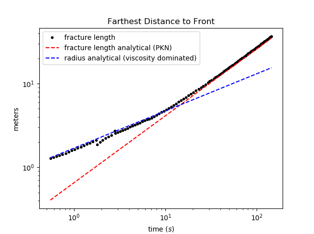
Expectedly, the solution first follows the viscosity dominated radial fracture solution and then transitions to height contained regime for which the classical PKN cite{PKN61} solution is applicable. The error introduced in the solution at about 2 seconds is due to re-meshing.

There are many fracture variables that we can plot now (you can see a list of variables that can be plotted in the Postprocessing and Visualization section). lets plot the footprint of the fracture in 3D and super impose the viscosity dominated and PKN analytical solutions. We will first load the saved fracture objects at the times at which we want to plot the footprint.

Fr_list, properties = load_fractures(address="./Data/height_contained",
                                     time_srs=np.asarray([1, 5, 20, 50, 80, 110, 140]))
time_srs = get_fracture_variable(Fr_list,
                                 variable='time')

Note that the fractures closest to the given times are loaded as the solutions are available only at the time steps at which the fractures were saved. The exact times are obtained from the loaded fracture list, at which the analytical solutions will be evaluated.

plot_prop_mesh = PlotProperties(text_size=1.7, use_tex=True)
Fig_Fr = plot_fracture_list(Fr_list,                           #plotting mesh
                            variable='mesh',
                            projection='3D',
                            backGround_param='sigma0',
                            mat_properties=properties[0],
                            plot_prop=plot_prop_mesh)

Fig_Fr = plot_fracture_list(Fr_list,                           #plotting footprint
                            variable='footprint',
                            projection='3D',
                            fig=Fig_Fr)

Fig_Fr = plot_analytical_solution('PKN',                       #plotting footprint analytical
                                  variable='footprint',
                                  mat_prop=Solid,
                                  inj_prop=Injection,
                                  fluid_prop=Fluid,
                                  fig=Fig_Fr,
                                  projection='3D',
                                  time_srs=time_srs[2:],
                                  h=7.0)
plt_prop = PlotProperties(line_color_anal='b')
Fig_Fr = plot_analytical_solution('M',
                                  variable='footprint',
                                  mat_prop=Solid,
                                  inj_prop=Injection,
                                  fluid_prop=Fluid,
                                  fig=Fig_Fr,
                                  projection='3D',
                                  time_srs=time_srs[:2],
                                  plot_prop=plt_prop)

plot_prop = PlotProperties(alpha=0.2, text_size=5)             #plotting width
Fig_Fr = plot_fracture_list(Fr_list,
                            variable='w',
                            projection='3D',
                            fig=Fig_Fr,
                            plot_prop=plot_prop)
ax = Fig_Fr.get_axes()[0]
ax.view_init(60, -114)

Fracture closure

In this example, we show the capability of PyFrac to handle fracture closure. The simulation consists of a 100 minutes injection of water into a rock with the following parameters

Paramters	Values
plane strain modulus	\(42.67\textrm{GPa}\)
fracture toughness	\(0.5\textrm{Mpa}\sqrt{\textrm{m}}\)
Carter’s leak off coefficient	\(10^{-6}\textrm{m}/\sqrt{\textrm{s}}\)
viscosity	\(1.1\times10^{-3}\textrm{Pa.s}\)
injection rate	\(0.001\textrm{m}^{3}/\textrm{s}\)
confining stress top & bottom layers	\(5.25\textrm{MPa}\)
confining stress middle layer	\(5\textrm{MPa}\)

The fracture is initiated in a layer that is bounded by layers having higher confining stress. The layer on top is set to have a small height, allowing the fracture to break through and accelerate upwards in another layer. We can proceed in the same manner as the previous examples. Lets make a mesh and define material, fluid and injection properties.

import numpy as np

# local imports
from mesh import CartesianMesh
from properties import MaterialProperties, FluidProperties, InjectionProperties, SimulationProperties

# creating mesh
Mesh = CartesianMesh(90, 66, 41, 27)

# solid properties
nu = 0.4                            # Poisson's ratio
youngs_mod = 4e10                   # Young's modulus
Eprime = youngs_mod / (1 - nu ** 2) # plane strain modulus
K_Ic = 5.0e5                        # fracture toughness

def sigmaO_func(x, y):
    """ This function provides the confining stress over the domain"""
    if 0 < y < 7:
        return 5.25e6
    elif y < -50:
        return 5.25e6
    else:
        return 5.e6

# material properties
Solid = MaterialProperties(Mesh,
                           Eprime,
                           toughness=K_Ic,
                           confining_stress_func=sigmaO_func,
                           Carters_coef=1e-6)

# injection parameters
Q0 = np.asarray([[0, 6000], [0.001, 0]])
Injection = InjectionProperties(Q0,
                                Mesh,
                                source_coordinates=[0, -20])

# fluid properties
Fluid = FluidProperties(viscosity=1e-3)

Note that we have provided coordinates of the injection point, which if not provided, are assumed to be at (0, 0). Next we will define the simulation properties. Since we expect to have fracture closure which is a stiffer problem, we increase the maximum number of iterations for the elasto-hydrodynamic solver and decrease the time step pre-factor.

from fracture import Fracture
from controller import Controller
from fracture_initialization import Geometry, InitializationParameters

# simulation properties
simulProp = SimulationProperties()
simulProp.finalTime = 1e5                       # the time at which the simulation stops
simulProp.set_outputFolder("./Data/fracture_closure") # the disk address where the files are saved
simulProp.bckColor = 'confining stress'         # setting the parameter for the mesh color coding
simulProp.plotTSJump = 4                        # set to plot every four time steps
simulProp.plotVar = ['w', 'lk', 'footprint']    # setting the parameters that will be plotted
simulProp.tmStpPrefactor = np.asarray([[0, 6000], [0.8, 0.4]]) # decreasing the time step pre-factor after 6000s
simulProp.maxSolverItrs = 120                   # increase maximum iterations for the elastohydrodynamic solver

# initialization parameters
Fr_geometry = Geometry('radial', radius=20)
init_param = InitializationParameters(Fr_geometry, regime='M')

# creating fracture object
Fr = Fracture(Mesh,
              init_param,
              Solid,
              Fluid,
              Injection,
              simulProp)

# create a Controller
controller = Controller(Fr,
                        Solid,
                        Fluid,
                        Injection,
                        simulProp)

# run the simulation
controller.run()

To visualize the results, lets first plot the fracture footprint at \(t=[240, 1028, 2211, 3322, 4644, 6000, 10388]\) seconds.

from visualization import *

# loading simulation results
time_srs = [230, 1000, 2200, 3200, 4500, 6000, 10388]
Fr_list, properties = load_fractures(address="./Data/fracture_closure",
                                     time_srs=time_srs)

# plot footprint
plt_prop = PlotProperties(color_map='Wistia', line_width=0.2)
Fig_FP = plot_fracture_list(Fr_list,
                            variable='mesh',
                            projection='2D',
                            mat_properties=Solid,
                            backGround_param='confining stress',
                            plot_prop=plt_prop
                            )
plot_prop1 = PlotProperties(plot_FP_time=False)
Fig_FP = plot_fracture_list(Fr_list,
                            variable='footprint',
                            projection='2D',
                            fig=Fig_FP,
                            plot_prop=plot_prop1)
Fig_FP.set_size_inches(5, 4)
plt.show(block=True)

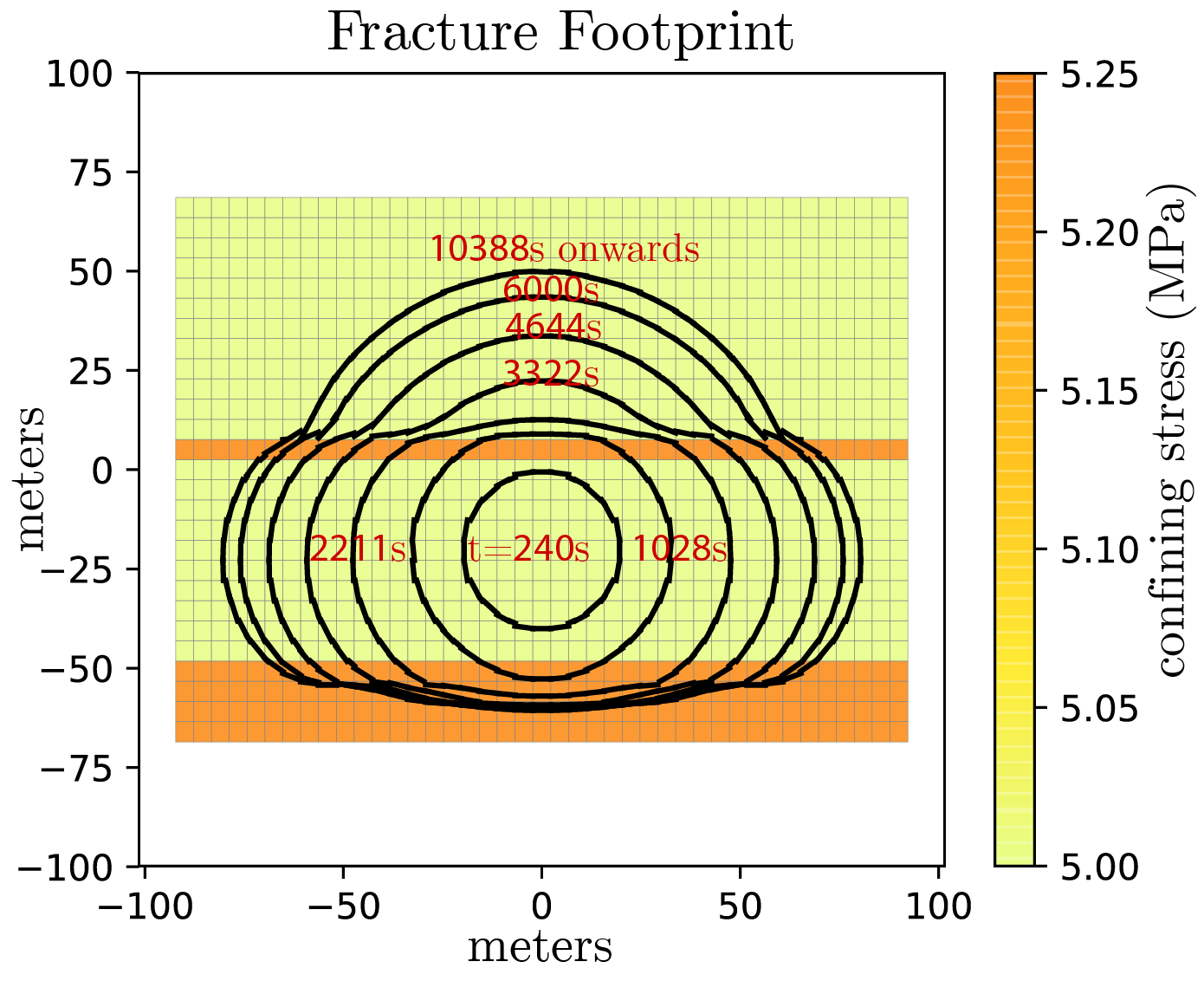
It can be seen that the fracture continues to slowly grow even after the injection has stopped at 6000s until it comes to a complete stop at 10388s. Due to fluid leak off, the fracture starts to close with time starting from 7672s. Lets animate the results to see the fracture propagating initially and then closing due to leak off.

Fr_list, properties = load_fractures(address="./Data/fracture_closure",
                                  time_srs=time_srs)

animate_simulation_results(Fr_list, ['w'])

Lateral spreading of a dyke at neutral buoyancy

This example demonstrates the capability of PyFrac to simulate buoyancy driven fractures. Here, we will simulate propagation of a dyke after a pulse injection of basaltic magma at a depth of 4.2Km. The magma fractures surrounding rock towards the surface as a dyke and hits a layer of less dense rock at a depth of 1.3Km, causing it to attain neutral buoyancy. As a result, the propagation is arrested vertically and the dyke spreads horizontally. We will use the following parameters taken from Traversa et al. - JGR-B (2010)

Paramters	Values
Young’s modulus	\(1.125\textrm{GPa}\)
fracture toughness	\(6.5\textrm{Mpa}\sqrt{\textrm{m}}\)
density of the rock (upper layer)	\(2300\textrm{Kg/m}^{3}\)
density of the rock (lower layer)	\(2700\textrm{Kg/m}^{3}\)
viscosity of magma	\(30\textrm{Pa.s}\)
density of magma	\(2400\textrm{Kg/m}^{3}\)
injection rate	\(2000\textrm{m}^{3}/\textrm{s}\)
time of injection	\(500\textrm{s}\)

We will set up the mesh and the material, fluid and injection properties in the same manner as we have done in the previous examples.

import numpy as np

# local imports
from mesh import CartesianMesh
from properties import MaterialProperties, FluidProperties, InjectionProperties, SimulationProperties

# creating mesh
Mesh = CartesianMesh(3200, 2800, 83, 83)

# solid properties
nu = 0.25                           # Poisson's ratio
youngs_mod = 1.125e9                # Young's modulus
Eprime = youngs_mod / (1 - nu ** 2) # plane strain modulus


def sigmaO_func(x, y):
    """ This function provides the confining stress over the domain"""
    density_high = 2700
    density_low = 2300
    layer = 1500
    Ly = 2800
    if y > layer:
        return (Ly - y) * density_low * 9.8
    # only dependant on the depth
    return (Ly - y) * density_high * 9.8 - (Ly - layer) * (density_high - density_low) * 9.8

# material properties
Solid = MaterialProperties(Mesh,
                           Eprime,
                           toughness=6.5e6,
                           confining_stress_func=sigmaO_func,
                           minimum_width=1e-5)

# injection parameters
Q0 = np.asarray([[0.0,  500],
                [2000,    0]])  # injection rate
Injection = InjectionProperties(Q0,
                                Mesh,
                                source_coordinates=[0, -1400])

# fluid properties
Fluid = FluidProperties(viscosity=30, density=2400)

# simulation properties
simulProp = SimulationProperties()
simulProp.finalTime = 560000                # the time at which the simulation stops
simulProp.set_outputFolder("./Data/neutral_buoyancy") # the disk address where the files are saved
simulProp.gravity = True                    # set up the gravity flag
simulProp.tolFractFront = 3e-3              # increase the tolerance for fracture front iteration
simulProp.plotTSJump = 4                    # plot every fourth time step
simulProp.saveTSJump = 2                    # save every second time step
simulProp.maxSolverItrs = 200               # increase the Picard iteration limit for the elastohydrodynamic solver
simulProp.tmStpPrefactor = np.asarray([[0, 80000], [0.3, 0.1]]) # set up the time step prefactor
simulProp.timeStepLimit = 5000              # time step limit
simulProp.plotVar = ['w', 'v']              # plot fracture width and fracture front velocity

Note that we have set the gravity flag to accommodate the effect of gravity. In addition, since the buoyancy driven fracture problem is more stiff, we have increase the maximum number of iterations for our solver to 200. To start the simulation, we will initialize a static radial fracture with a radius of \(300\textrm{m}\) and a net pressure of \(0.5\textrm{MPa}\). After the start of injection, the fracture will bloat like a balloon due to injection and pressure will increase. As it increases, the stress intensity factor at the tip will also increase until it will get equal to the fracture toughness of the rock. The fracture will start propagating at this stage. We will run the simulation through the controller just like the previous examples.

from fracture import Fracture
from controller import Controller
from fracture_initialization import Geometry, InitializationParameters
from elasticity import load_isotropic_elasticity_matrix

C = load_isotropic_elasticity_matrix(Mesh, Solid.Eprime)
Fr_geometry = Geometry('radial', radius=300)
nit_param = InitializationParameters(Fr_geometry,
                                   regime='static',
                                   net_pressure=0.5e6,
                                   elasticity_matrix=C)

Fr = Fracture(Mesh,
              init_param,
              Solid,
              Fluid,
              Injection,
              simulProp)

# create a Controller
controller = Controller(Fr,
                        Solid,
                        Fluid,
                        Injection,
                        simulProp)

# run the simulation
controller.run()

After the simulation is finished, we can plot the footprint and width of the fracture to visualize the results.

from visualization import *

# loading simulation results
time_srs = np.asarray([50, 350, 700, 1100, 2500, 12000, 50000, 560000])
Fr_list, properties = load_fractures(address="./Data/neutral_buoyancy",
                                     time_srs=time_srs)
time_srs = get_fracture_variable(Fr_list,
                                 variable='time')

# plot footprint
Fig_FP = None
Fig_FP = plot_fracture_list(Fr_list,
                            variable='mesh',
                            projection='2D',
                            mat_properties=Solid,
                            backGround_param='confining stress',
                            )
plt_prop = PlotProperties(plot_FP_time=False)
Fig_FP = plot_fracture_list(Fr_list,
                            variable='footprint',
                            projection='2D',
                            fig=Fig_FP,
                            plot_prop=plt_prop)

# plot width in 3D
plot_prop_magma=PlotProperties(color_map='jet', alpha=0.2)
Fig_Fr = plot_fracture_list(Fr_list[2:],
                            variable='width',
                            projection='3D',
                            plot_prop=plot_prop_magma
                            )
Fig_Fr = plot_fracture_list(Fr_list[1:],
                            variable='footprint',
                            projection='3D',
                            fig=Fig_Fr)

plt.show(block=True)